library(tidyverse)
library(readxl)ANOVA em DBC e parcela subdividida
Anova com bloco (DBC)
Preparo pré-análise:
Usando o conjunto de dados fungicida_campo:
fungicidas <- read_excel("dados-diversos.xlsx", "fungicida_campo")Modelo Anova com bloco
No delineamento em blocos, adiciona o sinal de + para adicionar a repetição.
aov_fung <- aov(sev ~trat + rep, data = fungicidas)
summary(aov_fung)
Df Sum Sq Mean Sq F value Pr(>F)
trat 7 7135 1019.3 287.661 <2e-16 ***
rep 1 19 18.6 5.239 0.0316 *
Residuals 23 81 3.5
---
Signif. codes: 0 '***' 0.001 '**' 0.01 '*' 0.05 '.' 0.1 ' ' 1Checando as premissas:
library(performance)
library(DHARMa)
check_normality(aov_fung)
OK: residuals appear as normally distributed (p = 0.230).check_heteroscedasticity(aov_fung)OK: Error variance appears to be homoscedastic (p = 0.484).plot(simulateResiduals(aov_fung))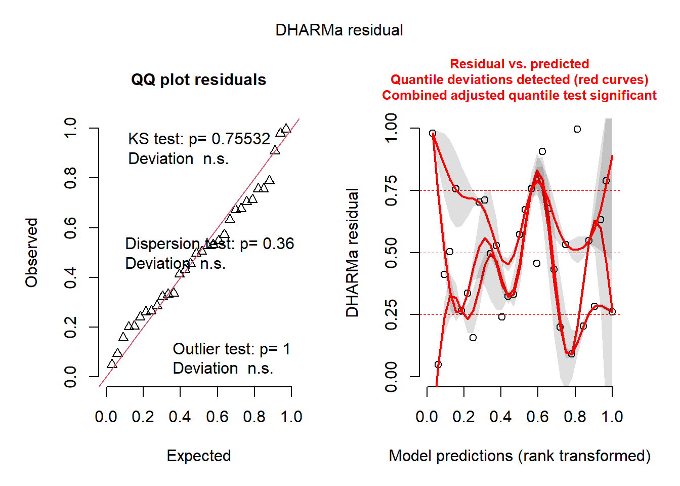
Estimando as médias:
library(emmeans)
means_fung <- emmeans(aov_fung, ~trat)
library(multcomp)
library(multcompView)
cld(means_fung)
trat emmean SE df lower.CL upper.CL .group
G 29.2 0.941 23 27.3 31.2 1
B 29.5 0.941 23 27.6 31.4 1
E 30.1 0.941 23 28.2 32.1 1
C 30.4 0.941 23 28.4 32.3 1
A 30.4 0.941 23 28.4 32.3 1
D 31.5 0.941 23 29.6 33.4 12
F 35.5 0.941 23 33.6 37.4 2
testemunha 75.8 0.941 23 73.8 77.7 3
Confidence level used: 0.95
P value adjustment: tukey method for comparing a family of 8 estimates
significance level used: alpha = 0.05
NOTE: If two or more means share the same grouping symbol,
then we cannot show them to be different.
But we also did not show them to be the same. plot(means_fung)+
coord_flip()+
theme_minimal()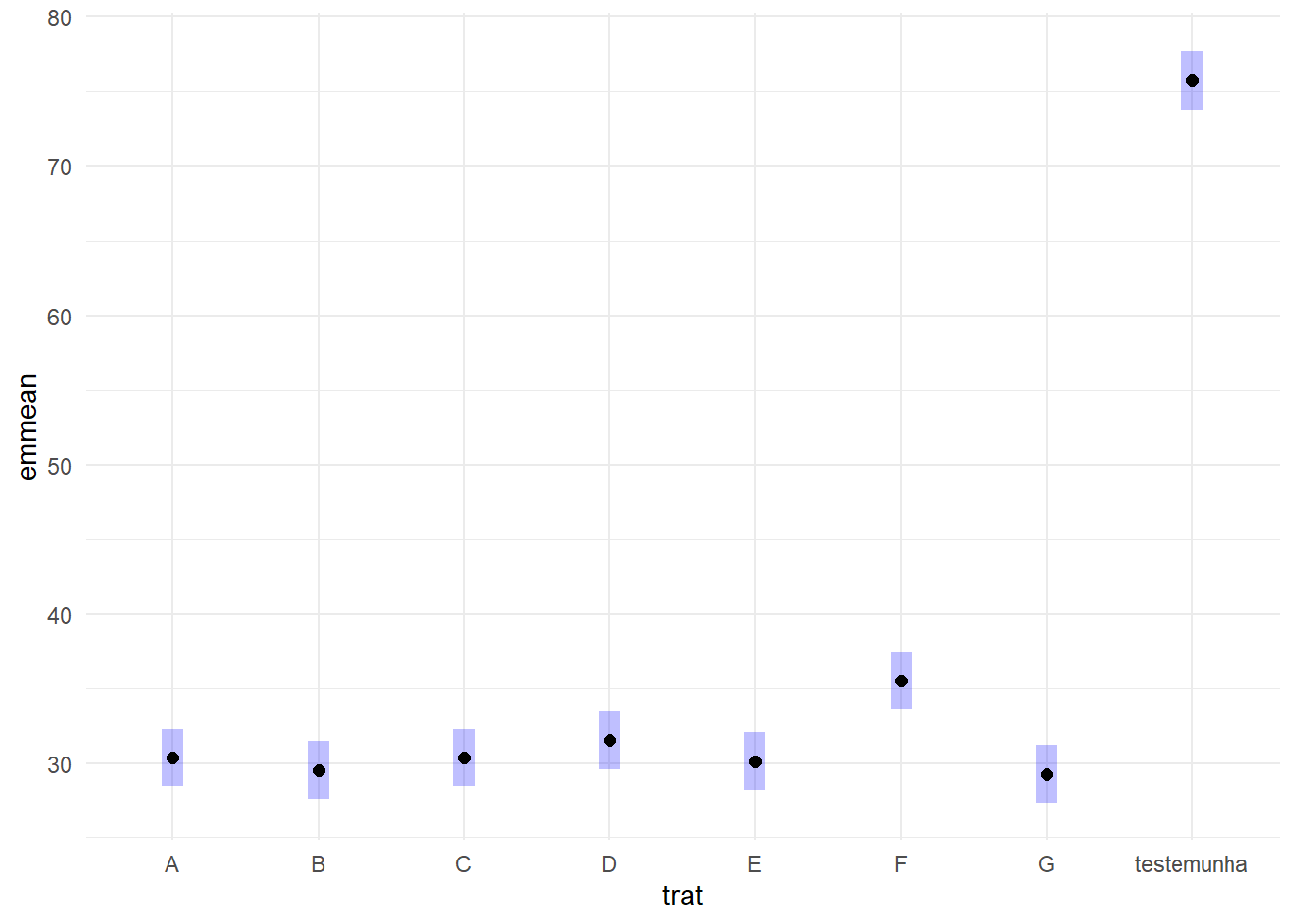
Delineamento em parcela subdividida (Split-plot)
Preparo pré-ánalise: usamos o conjunto milho,
milho <- read_excel("dados-diversos.xlsx", "milho")Ajustabndo o modelo:
aov_milho_bloco <- aov(index ~ factor(block) + hybrid*method +
Error(factor(block)/hybrid/method), data = milho)

summary(aov_milho_bloco)
Error: factor(block)
              Df Sum Sq Mean Sq
factor(block)  3  592.2   197.4

Error: factor(block):hybrid
          Df Sum Sq Mean Sq F value Pr(>F)
hybrid     5  974.2  194.84    3.14 0.0389 *
Residuals 15  930.9   62.06
---
Signif. codes:  0 '***' 0.001 '**' 0.01 '*' 0.05 '.' 0.1 ' ' 1

Error: factor(block):hybrid:method
              Df Sum Sq Mean Sq F value Pr(>F)
method         1  79.61   79.61   4.726 0.0433 *
hybrid:method  5 265.28   53.06   3.150 0.0324 *
Residuals     18 303.18   16.84
---
Signif. codes:  0 '***' 0.001 '**' 0.01 '*' 0.05 '.' 0.1 ' ' 1
Checa as premissas: Em parcelas subdivididas não é possível checar as premissas pelo check_, então usa lme4, para checar pelo modelo misto.
library(lme4)
milho$block <- as.factor(milho$block)
mix2 <- lmer(index ~ block + hybrid*method +
(1|block/hybrid), data =  milho)

library(car)
Anova(mix2)
Analysis of Deviance Table (Type II Wald chisquare tests)
Response: index
Chisq Df Pr(>Chisq)
block 0.3192 3 0.956380
hybrid 15.6987 5 0.007759 **
method 4.7262 1 0.029706 *
hybrid:method 15.7498 5 0.007596 **
---
Signif. codes: 0 '***' 0.001 '**' 0.01 '*' 0.05 '.' 0.1 ' ' 1check_normality(mix2)OK: residuals appear as normally distributed (p = 0.621).check_heteroscedasticity(mix2)Warning: Heteroscedasticity (non-constant error variance) detected (p = 0.009).Como os dados dão heterogneos, é necessário transformar os dados:
milho$block <- as.factor(milho$block)
mix2 <- lmer(sqrt(index) ~ block + hybrid*method + (1|block/hybrid), data = milho)
library(car)
Anova(mix2)
Analysis of Deviance Table (Type II Wald chisquare tests)
Response: sqrt(index)
Chisq Df Pr(>Chisq)
block 0.0764 3 0.994506
hybrid 15.4171 5 0.008721 **
method 3.9239 1 0.047605 *
hybrid:method 13.3025 5 0.020703 *
---
Signif. codes: 0 '***' 0.001 '**' 0.01 '*' 0.05 '.' 0.1 ' ' 1check_normality(mix2)OK: residuals appear as normally distributed (p = 0.422).check_heteroscedasticity(mix2)OK: Error variance appears to be homoscedastic (p = 0.970).Comparação de médias: Agora compara as médias, analisando a media para cada interação.
means_mix2 <- emmeans(mix2, ~hybrid | method)
means_mix2
method = pin:
hybrid emmean SE df lower.CL upper.CL
30F53 HX 5.00 1.17 5356 2.69 7.30
30F53 YH 4.95 1.17 5356 2.65 7.25
30K64 4.50 1.17 5356 2.20 6.81
30S31H 6.10 1.17 5356 3.79 8.40
30S31YH 5.63 1.17 5356 3.33 7.93
BG7049H 4.40 1.17 5356 2.10 6.71
method = silk:
hybrid emmean SE df lower.CL upper.CL
30F53 HX 4.94 1.17 5356 2.64 7.25
30F53 YH 5.10 1.17 5356 2.80 7.41
30K64 4.61 1.17 5356 2.31 6.91
30S31H 5.13 1.17 5356 2.83 7.43
30S31YH 5.14 1.17 5356 2.84 7.44
BG7049H 4.37 1.17 5356 2.07 6.67
Results are averaged over the levels of: block
Degrees-of-freedom method: kenward-roger
Results are given on the sqrt (not the response) scale.
Confidence level used: 0.95 cld(means_mix2)method = pin:
hybrid emmean SE df lower.CL upper.CL .group
BG7049H 4.40 1.17 5356 2.10 6.71 1
30K64 4.50 1.17 5356 2.20 6.81 1
30F53 YH 4.95 1.17 5356 2.65 7.25 12
30F53 HX 5.00 1.17 5356 2.69 7.30 12
30S31YH 5.63 1.17 5356 3.33 7.93 12
30S31H 6.10 1.17 5356 3.79 8.40 2
method = silk:
hybrid emmean SE df lower.CL upper.CL .group
BG7049H 4.37 1.17 5356 2.07 6.67 1
30K64 4.61 1.17 5356 2.31 6.91 1
30F53 HX 4.94 1.17 5356 2.64 7.25 1
30F53 YH 5.10 1.17 5356 2.80 7.41 1
30S31H 5.13 1.17 5356 2.83 7.43 1
30S31YH 5.14 1.17 5356 2.84 7.44 1
Results are averaged over the levels of: block
Degrees-of-freedom method: kenward-roger
Results are given on the sqrt (not the response) scale.
Confidence level used: 0.95
Note: contrasts are still on the sqrt scale
P value adjustment: tukey method for comparing a family of 6 estimates
significance level used: alpha = 0.05
NOTE: If two or more means share the same grouping symbol,
then we cannot show them to be different.
But we also did not show them to be the same. #Se quer comparar os 2 métodos dentro de cada hibrido:
#means_mix2 <- emmeans(mix2, ~ method | )
#means_mix2
#cld(means_mix2)